
Excel
Screen Layout

#
Spreadsheets
A spreadsheet is an electronic document that stores various types of
data. There are vertical columns and horizontal rows. A cell is
where the column and row intersect. A cell can contain data and can be
used in calculations of data within the spreadsheet. An Excel spreadsheet
can contain workbooks and worksheets. The workbook is the holder for
related worksheets.
# Ms Excel
It is the component of Ms-office XP which is
specially used to calculate mathematical calculation, data Manipulation and
analysis. File of Ms-Excel is called Workbook.
The file extension are:- .xlsx = work Book
Steps to open "Microsoft Excel" on computer
+ Click on Start button
+ Go on Run
+ Type excel
+ Click OK
or
+ Click on Start button
+ Click on Program
+ Click on Ms office
+ Click on Microsoft Excel 2007
#
Ribbon
Home: Clipboard, Fonts, Alignment, Number, Styles,
Cells, Editing
Insert: Tables, Illustrations, Charts, Links, Text
Page Layouts: Themes, Page Setup, Scale to Fit, Sheet Options,
Arrange
Formulas: Function Library, Defined Names, Formula Auditing,
Calculation
Data: Get External Data, Connections, Sort &
Filter, Data Tools, Outline
Review: Proofing, Comments, Changes
View: Workbook Views, Show/Hide, Zoom, Window, Macros
------------------------------------------------------------------------
Work book A excel work book is a file that
contain one or more worksheet which you can use to organize related
information.
Row: - Horizontal
group of cell is called row through 1 to 1048576.
Column: - Vertical
group of cell is called column through A to XFD.
Range The selected area of sheet is
called range.
Worksheet: -
The primary documents that you use in excel to store and work with data. It is
also called Spreadsheet. A work sheet contains number of cells that are
organized into column & rows.
No of Column
=16348
No of row=1048576.
Insert
Cells, Rows, and Columns
to insert cells, rows, and columns in Excel:
- Place the cursor in the row below where you want the
new row, or in the column to the left of where you want the new column
- Click the Insert
button on the Cells
group of the Home
tab
- Click the appropriate choice: Cell, Row, or Column

Delete
Cells, Rows and Columns
to delete cells, rows, and columns:
- Place the cursor in the cell, row, or column that
you want to delete
- Click the Delete
button on the Cells
group of the Home
tab
- Click the appropriate choice: Cell, Row, or Column

Find
and Replace
To find data or find and replace data:
- Click the Find
& Select button on the Editing group of the Home tab
- Choose Find
or Replace
- Complete the Find
What text box
- Click on Options
for more search options

Go To
Command
The Go To command takes you to a specific cell either by cell reference (the
Column Letter and the Row Number) or cell name.
- Click the Find
& Select button on the Editing group of the Home tab
- Click Go
To

Spell
Check
to check the spelling:
- On the Review
tab click the Spelling
button

Format
Worksheet Tab
You can rename a worksheet or change the color of the tabs to meet
your needs.
To rename a worksheet:
- Open the sheet to be renamed
- Click the Format
button on the Home
tab
- Click Rename
sheet
- Type in a new name
- Press Enter

To change the color of a worksheet tab:
- Open the sheet to be renamed
- Click the Format
button on the Home
tab
- Click Tab
Color
- Click the color

Reposition
Worksheets in a Workbook
To move worksheets in a workbook:
- Open the workbook that contains the sheets you want
to rearrange
- Click and hold the worksheet tab that will be
moved until an arrow appears in the left corner of the sheet
- Drag the worksheet to the desired
location

Insert
and Delete Worksheets
To insert a worksheet
- Open the workbook
- Click the Insert
button on the Cells
group of the Home
tab
- Click Insert
Sheet

To delete a worksheet
- Open the workbook
- Click the Delete
button on the Cells
group of the Home
tab
- Click Delete
Sheet

Copy
and Paste Worksheets:
To copy and paste a worksheet:
- Click the tab of the worksheet to be copied
- Right click and choose Move or Copy
- Choose the desired position of the sheet
- Click the check box next to Create a Copy
- Click OK

Getting satarted with
Function
A constant is a value that is not
calculated. For example, the date 10/9/2008, the number 210, and the text
"Quarterly Earnings" are all constants. An expression, or a value
resulting from an expression, is not a constant. If you use constant values in the
formula instead of references to the cells (for example, =30+70+110), the
result changes only if you modify the formula yourself.
Using calculation operators in formulas
Operators specify the type of
calculation that you want to perform on the elements of a formula. There is a
default order in which calculations occur, but you can change this order by
using parentheses.
Types of operators
There are four different types of
calculation operators
A.
Arithmetic operators
B.
Comparison operators
C.
text concatenation operators
D.
reference operators
1.
Arithmetic operators
To perform basic mathematical
operations such as addition, subtraction, or multiplication; combine numbers;
and produce numeric results, use the following arithmetic operators.
|
Arithmetic
operator |
Meaning |
Example |
|
+ (plus sign) |
Addition |
3+3 |
|
– (minus
sign) |
Subtraction
|
3–1 |
|
* (asterisk) |
Multiplication |
3*3 |
|
/
(forward slash) |
Division |
3/3 |
|
% (percent sign) |
Percent |
20% |
|
^
(caret) |
Exponentiation) |
3^2 |
2.
Comparison operators
You can compare two values with
the following operators. When two values are compared by using these oper
|
Comparison
operator |
Meaning |
Example |
|
= (equal sign) |
Equal to |
A1=B1 |
|
>
(greater than sign) |
Greater
than |
A1>B1 |
|
< (less than sign) |
Less than |
A1<B1 |
|
>=
(greater than or equal to sign) |
Greater
than or equal to |
A1>=B1 |
|
<= (less than or equal to sign) |
Less than or equal to |
A1<=B1 |
|
<>
(not equal to sign) |
Not
equal to |
A1<>B1 |
ators, the result is a logical
value either TRUE or FALSE.
3.
Text concatenation operator
Use the ampersand (&) to
join, or concatenate, one or more text strings to produce a single piece of
text.
|
Text
operator |
Meaning |
Example |
|
& (ampersand) |
Connects, or concatenates, two values to
produce one continuous text value |
"North"&"wind" |
4.
Reference operators
Combine ranges of cells for
calculations with the following operators.
|
Reference
operator |
Meaning |
Example |
|
: (colon) |
Range operator, which produces one reference
to all the cells between two references, including the two references |
B5:B15 |
|
,
(comma) |
Union
operator, which combines multiple references into one reference |
SUM(B5:B15,D5:D15) |
|
(space) |
Intersection operator, which produces on
reference to cells common to the two references |
B7:D7 C6:C8 |
Calculation order
Formulas calculate values in a
specific order. A formula in Excel always begins with an equal sign (=). The
equal sign tells Excel that the succeeding characters constitute a formula.
Following the equal sign are the elements to be calculated (the operands),
which are separated by calculation operators. Excel calculates the formula from
left to right, according to a specific order for each operator in the formula.
Operator precedence
If you combine several operators
in a single formula, Excel performs the operations in the order shown in the
following table. If a formula contains operators with the same precedence — for
example, if a formula contains both a multiplication and division operator —
Excel evaluates the operators from left to right.
|
Operator |
Description |
|
: (colon) (single
space) ,
(comma) |
Reference operators |
|
– |
Negation
(as in –1) |
|
% |
Percent |
|
^ |
Exponentiation |
|
* and / |
Multiplication and division |
|
+ and – |
Addition
and subtraction |
|
& |
Connects two strings of text (concatenation) |
|
= |
Comparison |
Use of parentheses
To change the order of evaluation,
enclose in parentheses the part of the formula to be calculated first. For
example, the following formula produces 11 because Excel calculates
multiplication before addition. The formula multiplies 2 by 3 and then adds 5
to the result.
=5+2*3
In contrast, if you use
parentheses to change the syntax, Excel adds 5 and 2 together and then
multiplies the result by 3 to produce 21.
=(5+2)*3
In the example below, the
parentheses around the first part of the formula force Excel to calculate B4+25
first and then divide the result by the sum of the values in cells D5, E5, and
F5.
=(B4+25)/SUM(D5:F5)
Using functions and nested
functions in formulas
Functions are predefined formulas
that perform calculations by using specific values, called arguments, in a
particular order, or structure. Functions can be used to perform simple or
complex calculations.
The
syntax of functions
The following example of the
ROUND function rounding off a number in cell A10 illustrates the syntax of a
function.

Structure of a function
![]() Structure. The structure of a function begins with an equal sign (=), followed
by the function name, an opening parenthesis, the arguments for the function
separated by commas, and a closing parenthesis.
Structure. The structure of a function begins with an equal sign (=), followed
by the function name, an opening parenthesis, the arguments for the function
separated by commas, and a closing parenthesis.
![]() Function name. For a list of available functions, click a cell and press
SHIFT+F3.
Function name. For a list of available functions, click a cell and press
SHIFT+F3.
![]() Arguments. Arguments can be numbers, text, logical values such as TRUE or
FALSE, arrays (array:
Used to build single formulas that produce multiple results or that operate on
a group of arguments that are arranged in rows and columns. An array range
shares a common formula; an array constant is a group of constants used as an
argument.), error values such as #N/A, or cell references (cell reference: The set of coordinates that a cell
occupies on a worksheet. For example, the reference of the cell that appears at
the intersection of column B and row 3 is B3.). The
argument you designate must produce a valid value for that argument. Arguments
can also be constants (constant:
A value that is not calculated and, therefore, does not change. For example,
the number 210, and the text "Quarterly Earnings" are constants. An
expression, or a value resulting from an expression, is not a constant.),
formulas, or other functions.
Arguments. Arguments can be numbers, text, logical values such as TRUE or
FALSE, arrays (array:
Used to build single formulas that produce multiple results or that operate on
a group of arguments that are arranged in rows and columns. An array range
shares a common formula; an array constant is a group of constants used as an
argument.), error values such as #N/A, or cell references (cell reference: The set of coordinates that a cell
occupies on a worksheet. For example, the reference of the cell that appears at
the intersection of column B and row 3 is B3.). The
argument you designate must produce a valid value for that argument. Arguments
can also be constants (constant:
A value that is not calculated and, therefore, does not change. For example,
the number 210, and the text "Quarterly Earnings" are constants. An
expression, or a value resulting from an expression, is not a constant.),
formulas, or other functions.
![]() Argument tooltip. A tooltip with the syntax and arguments appears as you type
the function. For example, type =ROUND( and the tooltip appears. Tooltips only
appear for built-in functions.
Argument tooltip. A tooltip with the syntax and arguments appears as you type
the function. For example, type =ROUND( and the tooltip appears. Tooltips only
appear for built-in functions.
Entering functions
When you create a formula that
contains a function, the Insert Function dialog box helps you enter
worksheet functions. As you enter a function into the formula, the Insert
Function dialog box displays the name of the function, each of its
arguments, a description of the function and each argument, the current result
of the function, and the current result of the entire formula.
To make it easier to create and
edit formulas and minimize typing and syntax errors, use formula autocomplete.
After you type an = (equal sign) and beginning letters or a display trigger,
Microsoft Office Excel displays below the cell a dynamic drop down list of
valid functions, arguments, and names that match the letters or trigger. You
can then insert an item in the drop-down list into the formula.
Nesting functions
In certain cases, you may need to
use a function as one of the arguments (argument:
The values that a function uses to perform operations or calculations. The type
of argument a function uses is specific to the function. Common arguments that
are used within functions include numbers, text, cell references, and names.) of
another function. For example, the following formula uses a nested AVERAGE
function and compares the result with the value 50.

![]() The
AVERAGE and SUM functions are nested within the IF function.
The
AVERAGE and SUM functions are nested within the IF function.
Valid returns
When a nested function is used as an argument, it must return the same type of
value that the argument uses. For example, if the argument returns a TRUE or
FALSE value, then the nested function must return a TRUE or FALSE. If it
doesn't, Microsoft Excel displays a #VALUE! error value.
Nesting level limits
A formula can contain up to seven levels of nested functions. When Function B
is used as an argument in Function A, Function B is a second-level function.
For instance, the AVERAGE function and the SUM function are both second-level
functions because they are arguments of the IF function. A function nested
within the AVERAGE function would be a third-level function, and so on.
List of functions
FUNCTIONS - Function are performed
formulas that perform calculation by using specific values in a particular
order or structure. Functions can be used to perform simple or complex
calculation. The structure of a function begins with an equal sign (=) followed
by the function name (sum) an opening parenthesis '(' the arguments (2, 3) for
the function separated by commas & a closing parenthesis ')'
Formula:- formula are equation that
perform calculation on values in your worksheet. A formula starts with an
equal sign (=) for example, the
following formula multiples 2 by 3 & than adds 5 to the results = 5+2*3
Formula bar:-A bar at the of the
excel window that you use to enter or edit values or formulas bar.
Following are the function.
A) Math & Trig function:
1) ABS:- returns the absolute value of
a number, a number without it's sign
Syntax:-
= Abs
(numbers)
=Abs (-2) gives absolute
value 2
2) Cos:- Returns the cosine of given angle.
Syntax:- = cos(numbers) = cos(60) - 1.047(98
number is the angle in radians for which you want
the cosine.
3) Degrees:- Converts radian into degree.
Syntax:- = degrees (angle)
Angle is the
angle in radians that you want to convert.
4) Power :-Returns the result of a
number roused to power.
Syntax:- =
power ( number, power)
= power
(5,2) ®
25 or 5^2 = 25
5) Product:- Multiplies all the numbers
given on arguments and return the products(Multiplication)
Syntax:-
=product(number 1, number 2)
6) Radians:- Convert degrees into
radian
Syntax:-
=Radian(angle)
Angle is an
angle in degree that you want to convert.
7) Round:- Round a number to a
specified number of a digits .
Syntax:- =round(numbers, number digits)
=round
(3.829,1) = 3.8
=round
(3.829,2) = 3.82
8) Sin:- Return the sin of the given
number.
Syntax:- =sin(number)
number is
the angle in radians for which you want the sin.
9) SQRT:- Return a positive square
root.
Syntax:- =SQRT(number)
number is
the number for which you want the square root.
=SQRT(16) =
4
10) SUM:- Adds all the numbers in a range a cells.
Syntax:- =SUM(number 1, number 2)
= SUM (A1:
A7)
11) Max:- Return maximum number of
cells.
Syntax:- =Max(number1, number2, ........... )
12) Min:- Return minimum number of
selected cells.
Syntax:- = Min(number1, number2, ........)
13) Count:- Count number in cells.
=count (number 1, number 2)
14) Average:- Return average of number.
=average (number 1, number 2)
Note:- 180 degrees = π * radians
B) Date and Time Function:
1) Date:- Return the number that
represent the date in ms-excel date time code.
Syntax:- =date (YY, MM, DD)
=date (30,
2, 23) = 2 / 23 / 1930
2) Now:- This function returns the
current date and time.
![]() Syntax:-
=now( )
Syntax:-
=now( )
=Today ( )
return date only.
Ctrl + :- =date Ctrl +
Shift +: = time
3) Time:- Return the number into time
Syntax:- =Time ( HH, MM, SS)
C) Logical Function:
1) If:- This function is checks whether a condition is met, return one
value. If true and another value if false
SYNTAX:-
= If (logical test, "value if
true", value if false)
Example:-
=If (A1>32, "Pass",
"Fail")
2) And:- This function check whether
all argument are true and return true, return false if any of argument is
false.
SYNTAX:-
=And (logical1,
logical2............)
Example:-
=If(And(C2>=32,
D2>=32.........) , "Pass", "Fail")
3) Or:- This function checks whether
any of the argument are true and return true return false only all argument are false.
SYNTAX:-
=Or(logical1, logical2)
Example:-
=If (or (C2<32, D2<32,
"Fail", "Pass")
Rank: - Return the rank of a number
from the list of number.
Syntax: - =Rank (number, reference)
![]() =Rank
(G3, G$3: G$10)
=Rank
(G3, G$3: G$10)
Conditional Formatting
Conditional Formatting: - This
is used to apply format to selected cells that meet specific criteria based on
formula you specify.
èSelect the cell range which is to be formatted.
èSelect the home tab
èclick on conditional formatting from styles group
ègo to highlight cells rules
èclick on more rules
èSelect the required formatting click on ok
Mordifing
Conditional Formatting:
èGo to conditional formatting
èSelect manage Rules
èmanage your formatting
èclick on ok
Data Vallidation
èData
Validation is used to prevent invalid data from being entered into a cell.
1) Select the range of cells that you wish to validate.
2) Click Data Tools group > Data Tab > Data Validation.
3) Click the Settings tab in the Data Validation
dialog box and specify the type of validation.
4) Check or uncheck the Ignore Blank checkbox to specify
what you want to do with the null values.
5) Optionally, arrange for an input message when the cell is clicked
6) Specify Excel’s response to the invalid data.
7) Click on Ok
Auto
filter
The quickest way to select only those
items you want to display in a list.
1.
Select
the data.
2.
From
data ribbon click on filter
3.
Click on drop down arrow and select the field
name from the list which you want display.
Removing Auto Filter
1.
From
data ribbon click on filter
Advanced
Filter
Filters data in a list so that only the rows that meet a
condition you specify by using a Criteria range is displayed.
Make the criteria for advance filter like
>60 at another cell.
1. Select the
data.
2. from data ribbon
click on advance filter.
3. Click on
copy another location.
4. Click on
list range box.
5. Enter
criteria range.
6. Enter the
range of data where u want to place filtered data
7. Click on ok.
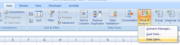
Goal Seek
Goal Seek: - This submenu adjusts the value in a specified cell until
a formula that is dependent on that cell reaches a target value. It can also be
define as Excel has a built-in tool called Goal
Seek, which is use to find the coefficient to the power law function.
Steps:-
èSelect a cell containig formula
èClick Data ribbon
èClick on what if analysis
èClick on Goal Seek
èA goal seek dialog box will appear
èSet cell which used to be changed, set target value
have to be in changed mode, give cell address which is used to be changed
èclick on OK
Define name
A name that represents a cell,
range of cells, formula, or constant value.
è Go to Formulas tab
èFrom the Defined Names group
èclick Define Names
èSet the name of the cell
èClick on ok
Define a name by using a
selection of cells in the worksheet
You can convert existing row and
column labels to names.
1.
Select the range that you want to name, including the row or
column labels.
2.
On the Formulas tab, in the Defined Names group,
click Create from Selection.

In the Create Names from Selection dialog box, designate the location
that contains the labels by selecting the Top row, Left column, Bottom
row, or Right column check box.
3.
Click on OK
Scenarios
Excel's
Scenario Manager is a tool that can be used to determine different
projected outcomes of data by changing different cells within a Worksheet
model.
· From the
top of Excel click the Data ribbon
· On the Data
menu, locate the Data Tools panel
· Click on
the What if Analysis item, and select Scenario Manager from the
menu:
· When you click Scenario
Manager, a scenario manager dialog box will appear:
· click the Add button. You'll then
get another dialogue box popping up:
· specify the
name of the scenario and changing cell range
· then
scenario values dialog box will appear
· specify the
values
· click on ok
· reapeat the
process upto your requirement
· then click the Summary to verify the report


Data Table
A
Data Table is a way to see different results by altering an input cell in your
formula. For example preparing a multiple table.
As:

From above figure:- Here cell A1 is the multiple
value of A12 and B12
· Select the data range as
above figure
· From the Excel ribbon, click
on Data tab
· Locate the Data Tools
panel
· Click on the "What if
Analysis" item:
· Then select data table
· a data table dialog box will
appear
· input the row input cell as
A12 and column input cell as B12
· then click on ok
The result is as

Example 2:
Consider
a case of compound interest, where
you invest a certain amount of money in a bank deposit and the amount is
compounded every year.
Formula
for calculating compound interest:
A
= P * (1 + r/n) ^ nt
Where:
- P = principal amount
(initial investment)
- r = annual interest rate
(as a decimal)
- n = number of times the
interest is compounded per year
- t = number of years
- A = amount after time t
Now,
if suppose we want to see what the final amount will be at different interests
rates, we can quickly use a data table for the same.
Excel Help describes a data table as:
A
data table is a range of cells that shows how changing one or two variables in
your formulas (formula: A sequence of values, cell references, names,
functions, or operators in a cell that together produce a new value. A formula
always begins with an equal sign (=).) will affect the results of those
formulas. Data tables provide a shortcut for calculating multiple results in
one operation and a way to view and compare the results of all the different
variations together on your worksheet.
Without
wasting any more time on descriptions, lets get down to creating a data table
for our compound interest example above.
Open
a new excel file and enter the following as given in the screenshot below:

The
cell B5 has the formula =B1 * (1 + B2) ^ B3
As
you can see, the $5000 invested at 7.5% for 5 years will give $7,178.15.
Now,
we will create a data table to see what amount we will receive by changing the
interest rate.
Fill
cells A6 to A10 with different interest rates. I’ve filled it with values from
6% to 10%. Now, select the cells A5:B10.

In
Excel 2007, goto Data > What-If Analysis > Data Table. In Excel
2003, the menu path is Data > Table or you can use the shortcut key Alt
+ D + T in this order.
This
will popup a window where you will be asked to enter Row Input Cell and the
Column Input Cell. Select the Column Input Cell as $B$2 and leave the
Row Input Cell blank and hit OK.

The
values will be filled in as shown below. You can choose to format them as
currency, but that I have left it upto you.

Chart
Charts allow you to present
information contained in the worksheet in a graphic format. Excel offers many
types of charts including: Column, Line, Pie, Bar, Area, Scatter and
more. To view the charts available click the Insert Tab on the Ribbon.

Create
a Chart
To create a chart:
- Select the cells that contain
the data you want to use in the chart
- Click the Insert tab on the
Ribbon
- Click the type of Chart you want to
create
Modify
a Chart
To modify the labels and titles:
- Click the Chart
- On the Layout tab, click the Chart
Title
or the Data Labels button
- Change the Title and click Enter
To change the data
included in the chart:
- Click the Chart
- Click the Select
Data
button on the Design tab
Chart
Tools
The Chart Tools appear on the Ribbon
when you click on the chart. The tools are located on three tabs:
Design, Layout, and Format.
èWithin the Design
tab you can control the chart type, layout, styles, and location.
èWithin
the Layout
tab you can control inserting pictures, shapes and text boxes, labels, axes,
background, and analysis.
èWithin the Format tab you can modify shape
styles, word styles and size of the chart.
|

|

|

To move the chart:
- Click the Chart and Drag it another
location on the same worksheet, or
- Click the Move
Chart
button on the Design tab
- Choose the desired location
(either a new sheet or a current sheet in the workbook)
Copy a
Chart to Word
- Select the chart
- Click Copy on the Home tab
- Go to the Word document where
you want the chart located
- Click Paste on the Home tab
Fomula auditing
Formula
Auditing is one of the Excel features that help you locate errors and display
their cell relationships

Trace Precedents
This option allows you to Identify, in a
visual manner, the Cells that are being Used In The Formula
of the cell that you have selected.
è Click on the cell that
contains the error
èthen click on the Trace Precedents Icon from the Formula Auditing
group. èExcel will trace the cell's
Precedents by drawing a Blue Arrow from the Precedent
Cell to Active Cell.
As:-

Trace
Dependents
This option allows you
to Identify Dependent Cells.
Dependent cells are the cells that use the values of other cells in their
calculations.
èSelect a Cell that is
being used in a formula,
èthen click
the Trace Dependents Icon on the Formula Auditing group
èExcel will
draw a Blue Arrow from the Active Cell to the Dependent Cell as shown in
the figure below.
To remove formula Auditing
èfrom the formula auditing group
èclick on remove arrows.
1.
On the Review tab, in the Changes group, click Protect
Workbook.

2.
Under Protect workbook for, do any of the following:
§ To protect
the structure of a workbook, select the Structure check box.
§ To keep
workbook windows in the same size and position each time the workbook is
opened, select the Windows check box.
Protect
worksheet elements
èOn the Review
tab, in the Changes group, click Protect Worksheet
èa protect
sheet dialog box will appear
èset the
password and chech the command which u want to alllow the user to modify
èclick on
Ok
èagain
confirm the password
èclick on
OK.
unprotect
worksheet elements
èopen the
document
ègo to review tab
èclick on unprotect
woeksheet.
èenter you password
èclick on ok
Protecting cell range
èSelect
the cell range
èclick on the Review tab
èselect “allow user to edit range”
èa “allow the user to edit range” dialog box will
appear
èclick on the new button
èa new
range dialogue box will appear
èset the
cell range and password
èclick on
ok and confirm the password again
èclick on
ok
èclick on ok


0 Comments